8 Basis of quantum algorithm

8.1 Review of basic concepts

8.1.1 Basic definitions

In physics, a quantum is the smallest inseparable basic unit of physical quantities. Bit, as a computer term, indicates the smallest unit of information. Different from a classical bit which can only be 0 or 1, a qubit can exist in the intermediate state superimposed in any proportion between 0 and 1.

The basic operation performed on qubits is called a quantum gate.

A quantum gate can either be a single-qubit gate and a multi-qubit gate. The single-qubit gate includes Hadamard gate, Pauli-X/Y/Z gate and rotating X/Y/Z gate. Two-qubit gates included controlled single-qubit gates (such as CNOT gates) and swap gates. A single-qubit gate and a two-qubit gate can be further extended to a multi-qubit gate by such extension means as controlled operation. It should be noted that measurement is a special quantum gate which is irreversible and changes the state of qubits.

Any quantum algorithm is a combination of these basic quantum gates.

See the common quantum logic gate matrix form for the definition of general quantum gate.

8.1.2 pyQPanda interface function

In pyQPanda the defined function of a quantum gate is as below:

gate = H(qubit)

Note

The input parameters are Qubit and other parameters, and the return value is QGate (quantum gate) which can be inserted into the quantum circuit.

Many kinds of quantum gates are defined in pyQPanda. Particularly, for the quantum gate U4 that supports full customization in pyQPanda, its interface functions supports simultaneous overloads as below:

As described above, the interface function of quantum gates is provided with two extension operations: transposed conjugate and controlled operation. Both of the operations can be implemented in two ways.

The two interface functions of transposed conjugate operation are defined as below:

gate = H(qubit)
gate1 = gate.dagger()
gate.setDagger(true)

Note

The dagger function returns a new quantum gate based on the target quantum gate, while the setDagger function returns the target quantum gate subject to transposed conjugate.

The two interface functions of controlled operation are defined as below:

gate = H(qubit)
gate1 = gate.control(QVec)
gate.setControl(QVec)

Note

The difference of controlled operation is similar to that of transposed conjugate operation, but the input parameter of the controlled operation function is Qvec (list of qubits) rather than a single qubit.

8.1.3 Example

Below is a program example to show the implementation of codes for basic qubit and quantum gate operations.

#!/usr/bin/env python

import pyqpanda as pq

if __name__ == "__main__":

    machine = pq.init_quantum_machine(pq.QMachineType.CPU)
    qubits = machine.qAlloc_many(3)
    control_qubits = [qubits[0], qubits[1]]
    prog = pq.create_empty_qprog()

    # Building quantum programs
    prog.insert(pq.H(qubits[0])) \
        .insert(pq.H(qubits[1])) \
        .insert(pq.H(qubits[0]).dagger()) \
        .insert(pq.X(qubits[2]).control(control_qubits))

    # Perform probability measurements on quantum programs
    result = pq.prob_run_dict(prog, qubits, -1)
    pq.destroy_quantum_machine(machine)

    # Print measurement results
    for key in result:
        print(key+":"+str(result[key]))

The output result shall be as shown below, with the probability of 0.5 to get \(|000⟩\) and \(|010⟩\):

0.4999999999999894
0.0
0.4999999999999894
0.0
0.0
0.0
0.0
0.0

Above is the basic definitions of qubit and quantum gate and the introduction to the call in pyQPanda.

8.2 Experimental state preparation and quantum entanglement

8.2.1 Experimental state preparation

Experimental state preparation refers to the construction of the initial quantum state of any algorithm in quantum computing, which is the initial step of quantum computing.

Taking the Space two-state space with a single qubit, in actual quantum computing, we can directly get the default quantum state as the ground state \(|0⟩\), and also get the ground state \(|1⟩\) indirectly through NOT gate.

For any given target superposition quantum state, we need to construct the corresponding combination of quantum gates to obtain such state. The process of preparing any given target superposition state by starting from the ground state \(|0⟩\) is known as the initial state preparation.

8.2.1.1 Maximum superposition state

Taking two-qubit state space as an example, we can get uniform superposition of all ground states in the two-qubit state space by performing Hadamard gate operation for each qubit, starting from \(|0⟩^{⊗2}\).

Similarly, in any dimensional state space, we can get the quantum state for uniform linear combinations of all ground states by starting from the multidimensional \(|0⟩\) ground state by virtue of Hadamard gate.

Such quantum state is called the maximum superposition state which is required by the initial state of qubits in many quantum computings. Also, the parallelism of quantum computing depends on such state.

Through the experimental state preparation, we can obtain any basic quantum state, thus completing the construction of operation objects in quantum computing. However, prior to the operation, we need to make clear constraint on the qubits used in quantum computing – entanglement and correlation.

We need to introduce pure state and mixed state before giving an introduction to quantum entanglement.

All quantum states rather than ground states are superposition states. Superposition states can be divided into coherent superposition and incoherent superposition which are called pure state and mixed state respectively.

Many methods are available to distinguish a pure state and a mixed state, including Bloch Sphere by which the state space is related to Bloch Sphere and the quantum state on the Sphere is a pure state while that in the Sphere is a mixed state.

Another important method is density matrix where the non-diagonal elements of the density matrix of mixed states are all 0.

8.2.2 Quantum entanglement

If the quantum state \(|ψ⟩\) of a quantum system can be expressed in the form of the direct product of two quantum systems like \(|ψ⟩=|ψ0 ⟩⊗|ψ1⟩\), such quantum state is called the direct product state.

Note

Any quantum state rather than direct product state is an entangled state.

For example, a two-qubit Bell state \(\frac{1}{\sqrt{2}}|00\rangle+\frac{1}{\sqrt{2}}|11\rangle\) cannot be factored as the direct product of two single-qubit quantum states.

The entangled state of quantum is given with quantum correlation beyond classical one. To give full play to the parallelism and efficiency of quantum computing, the qubits used in quantum computing shall be entangled and correlated.

8.2.3 Maximum superposition state preparation

The following is the code implementation for the maximum superposition state preparation based on pyQPanda, and the qubits called are entangled and correlated.

#!/usr/bin/env python

import pyqpanda as pq

if __name__ == "__main__":

    machine = pq.init_quantum_machine(pq.QMachineType.CPU)
    qubits = machine.qAlloc_many(3)
    prog = pq.create_empty_qprog()

    # Building quantum programs
    prog.insert(pq.H(qubits[0])) \
        .insert(pq.H(qubits[1])) \
        .insert(pq.H(qubits[2]))

    # Perform probability measurements on quantum programs
    result = pq.prob_run_dict(prog, qubits, -1)
    pq.destroy_quantum_machine(machine)

    # Print measurement results
    for key in result:
        print(key+":"+str(result[key]))

The results shall be that all quantum states in the 3-qubit space are obtained with the uniform probability of 1/8.

8.3 Hadamard Test and SWAP Test

A quantum circuit is a combination of a series of quantum gate operations. Among the numerous quantum circuits, some are used repeatedly during the construction of quantum algorithms. These frequently called quantum circuit components are called basic circuits of algorithm algorithms. Several common basic circuits will be introduced below.

8.3.1 Hadamard Test

The Hadamard Test quantum circuit is mainly used to give the projection and expectation \(⟨ψ|U|ψ⟩\) of any given unitary operator \(U\) on the given quantum state \(ψ\).

The quantum circuit diagram of Hadamard Test is simple in structure, as shown below.

The whole quantum circuit can be considered as the combination of quantum gate operations performed for the n+1-dimensional quantum state \(|0⟩|ψ⟩\) which is composed of qubits in two register \(\mathrm{Q}=\left(\mathrm{H} \otimes I^{\otimes n}\right)(\mathrm{C}-\mathrm{U})\left(\mathrm{H} \otimes I^{\otimes n}\right)\) where C−U represents a controlled gate based on the unitary operator U.

8.3.1.1 Output results and generalization

The derivation of the output results of Hadamard Test quantum circuit generates the following conclusions.

\[\begin{split}\begin{aligned} &\mathrm{Q}|0\rangle|\psi\rangle=\frac{|0\rangle+|1\rangle}{2}+\frac{|0\rangle-|1\rangle}{2} U|\psi\rangle \\ &=|0\rangle \frac{|\psi\rangle+\mathrm{U}|\psi\rangle}{2}+|1\rangle \frac{|\psi\rangle-\mathrm{U}|\psi\rangle}{2} \end{aligned}\end{split}\]

The probability to get \(|0⟩, |1⟩\) by measuring the output resulting quantum state is as below:

\[P_{0}=\frac{1}{4} \|(I+U)(\mathrm{Q}|0\rangle|\psi\rangle) \|^{2}=\frac{1+\operatorname{Re}(\langle\psi|U| \psi\rangle)}{2}, P_{1}=1-P_{0}\]

By deduced by the formula, the measurement probability of Hadamard Test results is related to the real part of \(Re(⟨ψ|U|ψ⟩)\) (unitary operator U) mapped and expected on the quantum state \(ψ\).

We can replace the H gate before the measurement with RX( :math:`frac{π}{2} ` ) gate to obtain the resulting quantum state related to the probability and the mapped and expected imaginary part.

8.3.1.2 Code example

A code of \(|\psi\rangle=\frac{|0\rangle+|1\rangle}{\sqrt{2}} \) , Hadamard Test is as below:

#!/usr/bin/env python

import pyqpanda as pq

if __name__ == "__main__":

        machine = pq.init_quantum_machine(pq.QMachineType.CPU)
        cqv = machine.qAlloc_many(1)
        tqv = machine.qAlloc_many(1)
        prog = pq.create_empty_qprog()

        # Building quantum programs
        prog.insert(pq.H(cqv[0])) \
                .insert(pq.H(tqv[0])) \
                .insert(pq.H(tqv[0]).control([cqv[0]]))\
                .insert(pq.H(cqv[0]))

        # Perform probability measurements on quantum programs
        result = pq.prob_run_dict(prog, cqv, -1)
        pq.destroy_quantum_machine(machine)

        # Print measurement results
        for key in result:
                print(key+":"+str(result[key]))

The output result shall be as shown below, with the probability of \(\frac{1+\sqrt{2} / 2}{2}\) and that of \(1-\frac{1+\sqrt{2} / 2}{2}\) to get \(|0⟩\) and \(|1⟩\) respectively:

0:0.853553
1:0.146447

Hadamard Test can be used for a wide range of purposes and has many forms among which one is basic SWAP Test of quantum circuits.

8.3.2 SWAP Test

With any two quantum states with the same dimension given, the fidelity of the two quantum states can be obtained through the SWAP Test circuit, which reflects the overlapping of the states.

The fidelity of the two quantum states refers to the square value of inner product norm of the quantum states, \(|⟨ϕ|ψ⟩|^2\)

The quantum circuit diagram of SWAP Test is as below.

The formula derivation and verification process for SWAP Test is completely similar to that for Hadamard Test, and the probability of \(|0⟩\), \(|1⟩\) measured by the first register for the resulting quantum state is related to the fidelity of the two given quantum states.

\[P_{0}=\frac{1+|\langle\psi \mid \phi\rangle|^{2}}{2}, P_{1}=1-P_{0}\]

SWAP Test, as a special form of Hadamard, provides the measurement results related to the fidelity for the two given quantum states, which shows significance of application. Also, it plays an important role in the study on inner product of quantum states.

If the controlled SWAP gate is replaced with a general controlled gate F, we can obtain the resulting quantum state of the general form of Hadamard Test.

\[\frac{|0\rangle}{2}(I+F)|\phi\rangle|\psi\rangle+\frac{|1\rangle}{2}(I-F)|\phi\rangle|\psi\rangle\]

8.3.2.1 Code example

There lies a minor difference between the code example of SWAP Test and that of Hadamard Test.

Take \(|\phi\rangle=\frac{|0\rangle+|1\rangle}{\sqrt{2}},|\psi\rangle=|1\rangle\) , an example of SWAP Test code is as below:

#!/usr/bin/env python

import pyqpanda as pq

if __name__ == "__main__":

    machine = pq.init_quantum_machine(pq.QMachineType.CPU)
    cqv = machine.qAlloc_many(1)
    tqv = machine.qAlloc_many(1)
    qvec = machine.qAlloc_many(1)
    prog = pq.create_empty_qprog()

    # Building quantum programs
    prog.insert(pq.H(cqv[0])) \
        .insert(pq.H(tqv[0])) \
        .insert(pq.X(qvec[0])) \
        .insert(pq.SWAP(tqv[0],qvec[0]).control([cqv[0]]))\
        .insert(pq.H(cqv[0]))

    # Perform probability measurements on quantum programs
    result = pq.prob_run_dict(prog, cqv, -1)
    pq.destroy_quantum_machine(machine)

    # Print measurement results
    for key in result:
        print(key+":"+str(result[key]))

The output result shall be as shown below, with the probabilities of 0.75 and 0.25 to get \(|0⟩\) and \(|1⟩\):

0:0.75
1:0.25

8.4 Amplitude magnification

The Amplitude Amplification circuit is mainly used to amplify the given pure state so as to adjust the probability distribution of its measured results.

8.4.1 Background of algorithm

For a finite set \(Ω\) of which the size is known and for which binary classification is available and standard \(f\) is determined by standard \(f\), any of element from the set \(|\Psi\rangle\) can be expressed as the linear combination of two orthogonal ground states \(\left|\Psi_{0}\right\rangle,\left|\Psi_{1}\right\rangle\) based on the \(f\).

\[|\psi\rangle=\sin \theta\left|\varphi_{1}\right\rangle+\cos \theta\left|\varphi_{0}\right\rangle,\left|\varphi_{0}\right\rangle=\left|\varphi_{1}^{\perp}\right\rangle\]

The amplitude amplification quantum circuit can amplify the amplitude of \(\left|\Psi_{1}\right\rangle\) in the expression of superposition state \(\left|\Psi\right\rangle\) , thus obtaining a resulting quantum state, so as to get the target quantum state \(\left|\Psi_{1}\right\rangle\) with a large probability.

Suppose that we can construct a combination of quantum gate operations which is the amplitude amplification operator Q, and we can obtain the quantum state in the following form by acting Q on the quantum state \(|\Psi\rangle\) for k times.

\[\left|\psi_{k}\right\rangle=\sin k \theta\left|\varphi_{1}\right\rangle+\cos k \theta\left|\varphi_{0}\right\rangle, k \theta \approx \frac{\pi}{2}\]

Then, we complete the required construction of amplitude amplification quantum circuits.

The quantum circuit diagram is as follows:

Suppose that the quantum state \(|\Psi\rangle\) based on the set \(Ω\) and classification standard \(f\) has been prepared, which depends on the construction of amplitude amplification operator \(Q\).

The amplitude amplification operator is defined as below:

\[P_{1}=I-2\left|\psi_{1}\right\rangle\left\langle\psi_{1}|, P=I-2| \psi\right\rangle\langle\psi|, Q=-P P_{1}\]

Note

How to prepare the quantum state through the set \(Ω\) and classification standard \(f\)? How are \(P_{1}\) and \(P\) implemented through the quantum circuit?

Through simple verification, we can know that the operation \(Q\) in the space formed by \(\left\{\left|\varphi_{1}\right\rangle,\left|\varphi_{0}\right\rangle\right\}\) can be expressed as follows:

\[\begin{split}Q=\left[\begin{array}{cc} \cos (2 \theta) & -\sin (2 \theta) \\ \sin (2 \theta) & \cos (2 \theta) \end{array}\right]\end{split}\]

Essentially, it can be considered as a rotating quantum gate operation with an angle of \(2θ\). Therefore, we can get the following formula:

\[Q^{n}|\psi\rangle=\sin (2 n+1) \theta\left|\varphi_{1}\right\rangle+\cos (2 n+1) \theta\left|\varphi_{0}\right\rangle\]

The amplitude amplification quantum circuit can be completed by selecting a proper number of rotation n to make \(\sin ^{2}(2 n+1) \theta\) be closest to 1.

Compared with the classical traversal classification method, the amplitude amplification quantum circuit can fully reflect the advantages of quantum computing.

8.4.2 Code example

Take \(\Omega=\{0,1\},|\psi\rangle=\frac{|0\rangle+|1\rangle}{2}, P_{1}=I-2|1\rangle\langle 1|=Z\)

Below is an example of codes corresponding to the amplitude amplification quantum circuit:

#!/usr/bin/env python

import pyqpanda as pq
from numpy import pi

if __name__ == "__main__":

    machine = pq.init_quantum_machine(pq.QMachineType.CPU)
    qvec = machine.qAlloc_many(1)
    prog = pq.create_empty_qprog()

    # Building quantum programs
    prog.insert(pq.H(qvec[0]))
    for i in range(7):
         prog.insert(pq.RY(qvec[0],pi/2))

    # Perform probability measurements on quantum programs
    result = pq.prob_run_dict(prog, qvec, -1)
    pq.destroy_quantum_machine(machine)

    # Print measurement results
    for key in result:
         print(key+":"+str(result[key]))

The output result shall be as shown below, with the probabilities of \(1\) and \(0\) to get \(|0⟩\) and \(|1⟩\) respectively:

0:1
1:0

8.5 Quantum Fourier transform

The quantum Fourier transform (QFT) is the quantum version of the classical inverse discrete Fourier transform.

The quantum Fourier transform converts the data in the base vector to the data in the amplitude under certain conditions and vice versa.

8.5.1 Basic definition

QFT can be obtained by simply substituting IDFT. Both QFT and DFT are essentially different forms of expression of the same vector in two equivalent spaces, i.e., the substitution of base vectors.

\[\begin{split}\begin{aligned} y_{k} & \rightarrow \frac{1}{\sqrt{N}} \sum_{j=0}^{N-1} x_{j} e^{\frac{2 \pi i}{N} j k} \\ |x\rangle & \rightarrow \frac{1}{2^{\frac{n}{2}}} \Sigma_{k=0}^{2^{n}-1} e^{\frac{2 \pi i}{2^{n}} x k}|k\rangle \end{aligned}\end{split}\]

Based on the definition, a certain vector \(\Sigma_{x} \alpha_{x}|\mathrm{x}\rangle\) in the space \(span{|x⟩}\) can be represented as the linear combination \(\Sigma_{k} \beta_{k}|k\rangle\) of base vectors in another equivalent space \(span{|k⟩}\) through Fourier transform, and the coefficient \(\beta_{k}\) of the linear combination depends on \(|x⟩\) and \(\alpha_{k}\) .

Note

The quantum Fourier transform/inverse transform can be essentially considered as a mutual transformation of amplitude and base vector.

8.5.2 Construction of quantum circuit

The implementation of quantum circuits of QFT requires the transformation of its expression to obtain the transformation process which can be implemented with the existing general quantum gate combination.

8.5.2.1 Sum form and tensor product form of QFT

By any given integer \(x\), \(k=\Sigma_{i=1}^{n} k_{i} 2^{n-i}\) is expanded by the binary system, and the result of quantum Fourier transform of \(|x⟩\) can be expressed as below:

\[\begin{split}\begin{aligned} &Q F T(|x\rangle)=\frac{1}{2^{\frac{n}{2}}} \Sigma_{k=0}^{2^{n}-1} e^{\frac{2 \pi i i x k}{2^{n}}}|k\rangle=\frac{1}{2^{\frac{n}{2}}} \Sigma_{k_{1}=0}^{1} \cdots \Sigma_{k_{n}=0}^{1} e^{2 \pi i x k\left(\Sigma_{L}^{n} k l^{2}-\right)}\left|k_{1} \cdots k_{n}\right\rangle \\ &=\frac{1}{2^{\frac{n}{2}}} \Sigma_{k_{1}=0}^{1} \cdots \Sigma_{k_{n}=0}^{1} \otimes_{l=1}^{n} e^{2 \pi i x k l^{-l}}\left|k_{l}\right\rangle=\frac{1}{2^{\frac{n}{2}}} \otimes_{l=1}^{n}\left(|0\rangle+e^{2 \pi i x 2^{-l}}|1\rangle\right) \end{aligned}\end{split}\]

As shown by the above formula, QFT can express the particular quantum state \(|x⟩\) as a linear combination of another set of base vectors, and such linear combination can also be expressed as the tensor product of multiple single-qubit states \(\frac{1}{\sqrt{2}}\left(|0\rangle+e^{2 \pi i x 2^{-l}}|1\rangle\right)\) .

Therefore, for any given integer \(x\), we, if able to construct a quantum state \(\frac{1}{\sqrt{2}}\left(|0\rangle+e^{2 \pi i x 2^{-l}}|1\rangle\right)\) with binary expansion qubits, can complete the construction of corresponding QFT quantum circuits through the QFT expression in the form of tensor product.

8.5.2.2 Binary expansion and quantum state preparation

Binary expansion approximation for any given integer \(x\):

\[\frac{\mathrm{x}}{2^{m}} \approx \frac{\left[x_{1} \ldots x_{m}\right]}{2^{m}}=\left[0 . x_{1} \ldots x_{m}\right]=\sum_{k=1}^{m} x_{k} 2^{-k}\]

while

\[ \begin{align}\begin{aligned} 2 \pi \mathrm{ix} 2^{-l}=2 \pi i\left[x_{1} \ldots x_{n}\right] 2^{-l}=2 \pi i\left[0 . x_{n-l} \ldots x_{n}\right]\\Then, the preparation of\end{aligned}\end{align} \]

\(\frac{1}{\sqrt{2}}\left(|0\rangle+e^{2 \pi i x 2^{-l}}|1\rangle\right)\) is transformed into that of \(\frac{1}{\sqrt{2}}\left(|0\rangle+e^{2 \pi i\left[0 . x_{n-l} \ldots x_{n}\right]}|1\rangle\right)\)

It shall be noted that \(\mathrm{H}|0\rangle=\frac{1}{\sqrt{2}}(|0\rangle+|1\rangle)=\frac{1}{\sqrt{2}}\left(|0\rangle+e^{2 \pi i\left[0 . x_{n}\right]}|1\rangle\right)\) while

\[\begin{split}\begin{gathered} \frac{1}{\sqrt{2}}\left(|0\rangle+e^{2 \pi i\left[0 x_{n-l} \ldots x_{n}\right]}|1\rangle\right)=\frac{1}{\sqrt{2}}\left(|0\rangle+e^{2 \pi i\left[0 . x_{n-1}\right]} e^{2 \pi i\left[0 . x_{n}\right]}|1\rangle\right) \\ R_{m}|0\rangle=|0\rangle, \quad R_{m}|1\rangle=e^{2 \pi i \frac{1}{2^{m}}}|1\rangle \end{gathered}\end{split}\]

The defined controlled rotating quantum gate \((\mathrm{C}-\mathrm{R})_{j-k+1}\) meets

\[ \begin{align}\begin{aligned} (\mathrm{C}-\mathrm{R})_{j-k+1} \frac{1}{\sqrt{2}}\left(|0\rangle+e^{2 \pi i\left[0 . x_{n-j}\right]}|1\rangle\right)\left|x_{n-k}\right\rangle=\frac{1}{\sqrt{2}}\left(|0\rangle+e^{2 \pi i\left[0 . x_{n-j}\right]}|1\rangle\right)\\Therefore, the preparation of quantum state\end{aligned}\end{align} \]

\(\frac{1}{\sqrt{2}}\left(|0\rangle+e^{2 \pi i x 2^{-l}}|1\rangle\right)\) can be achieved by using quantum gate H and \((\mathrm{C}-\mathrm{R})_{j-k+1}\) thus completing the quantum circuit of QFT.

The quantum circuit diagram of QFT is as below.

In particular, we have noticed that the resulting quantum state corresponding to the qubit with the initial quantum state being \(\left|\mathrm{x}_{i}\right\rangle\) is \(\frac{1}{\sqrt{2}}\left(|0\rangle+e^{2 \pi i x 2^{n+1-l}}|1\rangle\right)\) instead of \(\frac{1}{\sqrt{2}}\left(|0\rangle+e^{2 \pi i x 2^{-l}}|1\rangle\right)\) . Thus, we need add multiple sets of SWAP gates in actual applications.

8.5.3 Code implementation

QFT in one dimension is a Hadamard quantum gate. The QFT interface function based on pyQPanda is as below:

QFT(qlist)

The example where \(|x⟩=|000⟩\) is taken to verify the code example of QFT is as below:

#!/usr/bin/env python

import pyqpanda as pq
from numpy import pi

if __name__ == "__main__":

    machine = pq.init_quantum_machine(pq.QMachineType.CPU)
    qvec = machine.qAlloc_many(3)
    prog = pq.create_empty_qprog()

    # Building quantum programs
    prog.insert(pq.QFT(qvec))

    # Perform probability measurements on quantum programs
    result = pq.prob_run_dict(prog, qvec, -1)
    pq.destroy_quantum_machine(machine)

    # Print measurement results
    for key in result:
         print(key+":"+str(result[key]))

According to the definition of QFT as given above and \(|x⟩=|000⟩\), the output result be all the quantum states obtained based on the uniform probability of 1/8, i.e.:

8.6 Quantum phase estimation

Quantum phase estimation (QPE) can serve to compute the phase of the eigenvalue of a given unitary operator (U), i.e., solve φ in \(\mathrm{U}|\psi\rangle=e^{2 \pi i \varphi}|\psi\rangle \text { where }|\Psi\rangle\) is the eigenvector of U.

The QPE in classical form is constructed on the basis of QFT

8.6.1 Overview of structure of quantum circuit

Suppose that the eigenvector \(|\Psi\rangle\) has been constructed. Quantum phase estimation includes the steps below:

1.The eigenvalue phase of U is decomposed and transferred to the amplitude of the auxiliary qubit through a series of special rotating quantum gate operations.

2.IQFT is conducted for the auxiliary qubit to transfer the decomposed eigenvalue phases on the amplitude to the base vectors.

3.The phase information of the eigenvalue can be obtained by measuring the base vectors of the auxiliary qubit.

For an eigen quantum state \(|\Psi\rangle\) of the unitary operator U, we can extract the eigenvalue phase corresponding to the quantum state to the amplitude through specific quantum gate combination, but it is hard to accurately and effectively measure the amplitude of the quantum state.

We have to integrate the eigenvalue phase data by virtue of quantum gate combinations, and can transfer the eigenvalue to the base vector by taking advantage of the function of IQFT to transfer amplitude to base vector.

Note

Quantum phase estimation is essentially used to extract the eigenvalue phases of unitary operators and output the phases in a form convenient for measurement.

8.6.2 Construction of quantum circuit

8.6.2.1 Eigen quantum state and eigenvalue phase extraction

According to the definition of eigen quantum state \(\mathrm{U}|\psi\rangle=e^{2 \pi i \varphi}|\psi\rangle\)

Therefore, the unitary operator U can define a controlled quantum gate (C−U) to enable

\[\left(\mathrm{C}-U^{2^{t}}\right)(\mathrm{a}|0\rangle+\mathrm{b}|1\rangle) \otimes|\psi\rangle=\left(\mathrm{a}|0\rangle+e^{2 \pi i \varphi 2^{t}} \mathrm{~b}|1\rangle\right) \otimes|\psi\rangle\]

The eigenvalue phase \(\psi\ \) can be extracted into the amplitude through such controlled transformation.

8.6.2.2 Transfer of eigenvalue phase from amplitude to base vector

We select a set of auxiliary qubits which are initialized to the maximum superposition state, and can extract the eigenvalue phase into the amplitude through the controlled quantum gate:

\[\left(\mathrm{C}-U^{2^{\circ}}\right) \ldots\left(\mathrm{C}-U^{2^{n}}\right) \frac{1}{2^{\frac{n}{2}}} \otimes_{t=1}^{n}(|0\rangle+|1\rangle)=\left(|0\rangle+e^{2 \pi i \varphi 2^{1-1}}|1\rangle\right) \ldots\left(|0\rangle+e^{2 \pi i \varphi 2^{n-1}}|1\rangle\right)\]

At this point, the form of quantum state in the auxiliary qubits is close to that of the resulting quantum state of QFT, and the following results can be obtained with the help of IQFT:

\[\begin{split}\begin{aligned} &\mathrm{QFT}^{-1} \frac{1}{2^{\frac{n}{2}}} \otimes_{t=1}^{n}\left(|0\rangle+e^{2 \pi i \varphi 2^{t-1}}|1\rangle\right) \\ &=\mathrm{QFT}^{-1} \frac{1}{2^{\frac{n}{2}}} \sum_{k=0}^{2^{n}-1} e^{2 \pi i \varphi k}|\mathrm{k}\rangle \\ &=\frac{1}{2^{n}} \sum_{k=0}^{2^{n}-1} \sum_{x=0}^{2^{n}-1} e^{-\frac{2 \pi i k}{2^{n}}\left(x-2^{n} \varphi\right)}|\mathrm{x}\rangle \end{aligned}\end{split}\]

The quantum state obtained is measured and the measurement results can be divided into the two following categories:

1.Where the positive integer \(2^{n} \varphi \in Z\) is available, can be obtained through measurement with a probability of \(|\mathrm{x}\rangle=\left|2^{n} \varphi\right\rangle\) .

2.Otherwise, with probability of \(\frac{4}{\pi^{2}}\) , we can obtain the integer which is closest to \(2^{n} \varphi\) , thus to obtain the approximate solution.

from the integer which is closest to \(2^{n} \varphi\) ? (Tip: continued fraction expansion)

The measurement result is the approximate solution of phase \(\varphi\) of which the precision is related to the number of auxiliary qubits n. \(2^{n} \varphi \in Z\) indicates that the number of auxiliary qubits is already greater than that of binary expansion decimal places of \(\varphi\) so that the exact solution can be gotten.

8.6.3 Quantum circuit diagram and code implementation

The quantum circuit diagram of QPE is as below.

As disclosed by the above definition, we can provide the function implementation of QPE directly based on QPanda-2.0.

The quantum circuit can be divided into three parts, namely, eigen quantum state preparation, auxiliary qubit quantum state initialization, eigenvalue phase extraction and inverse quantum Fourier transform. The core contents of the program implementation are as follows:

#!/usr/bin/env python

import pyqpanda as pq
from numpy import pi

def QPE(controlqlist, targetqlist, matrix):
   circ = pq.QCircuit()
   for i in range(len(controlqlist)):
          circ.insert(pq.H(controlqlist[i]))
   for i in range(len(controlqlist)):
          circ.insert(controlUnitaryPower(targetqlist, controlqlist[controlqlist.size() \
           - 1 - i], i, matrix))

   circ.insert(pq.QFT(controlqlist).dagger())
   return circ

The parameter matrix in the figure refers to the matrix corresponding to the unitary operator U requiring eigenvalue estimation.

When \(\mathrm{U}=\operatorname{RY}\left(\frac{\pi}{4}\right),|\psi\rangle=|0\rangle+\mathrm{i}|1\rangle\) is selected, the eigenvalue is \(e^{-i \frac{\pi}{8}}\) and the code example for QPE verification is as below.

#!/usr/bin/env python

import pyqpanda as pq
from numpy import pi

if __name__ == "__main__":

   machine = pq.init_quantum_machine(pq.QMachineType.CPU)
   qvec = machine.qAlloc_many(1)
   cqv = machine.qAlloc_many(2)
   prog = pq.create_empty_qprog()

   # Building quantum programs
   prog.insert(pq.H(cqv[0]))\
         .insert(pq.H(cqv[1]))\
         .insert(pq.S(qvec[0]))\
         .insert(pq.RY(qvec[0], pi/4).control(cqv[1]))\
         .insert(pq.RY(qvec[0], pi/4).control(cqv[0]))\
         .insert(pq.RY(qvec[0], pi/4).control(cqv[0]))\
         .insert(pq.QFT(cqv).dagger())

   # Perform probability measurements on quantum programs
   result = pq.prob_run_dict(prog, cqv, -1)
   pq.destroy_quantum_machine(machine)

   # Print measurement results
   for key in result:
         print(key+":"+str(result[key]))

As implied above, the output result should be the quantum state \(|0⟩\) with a large probability

000, 0.821067
001, 0.0732233
010, 0.0324864
011, 0.0732233

8.7 For operations of quantum

In particular cases, four basic operations shall be implemented in a quantum computer. The quantum adder and the four operations of quantum derived therefrom can meet the computing requirements

8.7.1 Background of adder algorithm

All quantum gate operations except measurement are unitary transformations, and thus the quantum circuit excluding measurement is reversible as a whole.

The quantum circuit of a quantum adder shall also be reversible, so that the inputs and outputs are an equal number of qubits. The quantum circuit diagram is shown below.

The figure above contains two quantum circuit modules MAJ and UMA which mainly serve to obtain the carry value and resulting value of the current binary qubit.

8.7.1.1 Component of MAJ quantum circuit

The quantum circuit diagram of MAJ is as below.

The specific functions of MAJ quantum circuits are explained as follows.

The inputs of MAJ quantum circuits are the carry value \(\mathrm{c}_{i}\) of the previous qubit and the two values to be added (\(\mathrm{a}_{i}\) and \(\mathrm{b}_{i}\) ) of the current qubit while the outputs are \(\mathrm{a}_{i}+\mathrm{c}_{i}\) mod 2, \(\mathrm{a}_{i}+\mathrm{b}_{i}\) mod 2 and the carry value \(\mathrm{c}_{i+1}\) of the current qubit.

The MAJ module is to achieve carry bits. We want to get carry qubit \(\mathrm{c}_{i+1}\) , i.e., judge \(\left(a_{i}+b_{i}+c_{i}\right) / 2\) by starting from \(\left(a_{i}+b_{i}+c_{i}\right)\).

We select a number \(\mathrm{a}_{i}\) from the values to be added to enumerate the carry bits as follows:

\[\begin{split}\begin{aligned} &\text { 1. } a_{i}=0, \quad c_{i}=\left[\left(a_{i}+b_{i}\right) \% 2\right] *\left[\left(a_{i}+c_{i}\right) \% 2\right]; \\ &\text { 2. } a_{i}=1, \quad c_{i}=\left(\left[\left(a_{i}+b_{i}\right) \% 2\right] *\left[\left(a_{i}+c_{i}\right) \% 2\right]+1\right) \% 2 ; \end{aligned}\end{split}\]

Therefore, we can judge the carry bits by only studying \(\mathrm{a}_{i}\)，

\[\left[\left(a_{i}+b_{i}\right) \% 2\right] *\left[\left(a_{i}+c_{i}\right) \% 2\right]\]

We can accurately judge the carry bits by starting from the existing quantum logic gate and preparing the quantum state \(\mathrm{a}_{i}\),\(\left[\left(a_{i}+b_{i}\right) \% 2\right] ,\left[\left(a_{i}+c_{i}\right) \% 2\right]\).The subject of study selected here is not unique. Other schemes will result in corresponding quantum circuits.

The scheme for preparing three quantum states is shown in the figure above. We use CNOT gate to complete module 2 addition to obtain \(\left(a_{i}+b_{i}\right) \% 2\)，\(\left(a_{i}+c_{i}\right) \% 2\),and Toffoli gate to complete the XOR operation of a and \(\left[\left(a_{i}+b_{i}\right) \% 2\right] *\left[\left(a_{i}+c_{i}\right) \% 2\right]\).

8.7.1.2 Component of UMA quantum circuit

The quantum circuit diagram of UMA is as below.

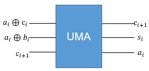
The specific functions of UMA quantum circuits are explained as follows.

The inputs of UMA quantum circuits are \(a_{i}+c_{i} \bmod 2, a_{i}+b_{i} \bmod 2\) , and the carry value \(c_{i+1}\) of the current bit while the outputs are \(c_{i}, \mathrm{a}_{i}+\mathrm{b}_{i}+c_{i} \bmod 2:=\mathrm{s}_{i} \text { and } \mathrm{a}_{i}\) .

The UMA module is to achieve the results of current bits. We want to get current bit \(\mathrm{s}_{i}\) ,i.e., \(\left(a_{i}+b_{i}+c_{i}\right) \% 2\)

By referring to the MAJ module, we get \(a_{i}\) from \(c_{i+1}\) through the TOffoli gate which is \(c_{i+1}\) through Toffoli gate which is completely opposite to that used by MAJ, and then get \(c_{i}\) through CNOT transformation which is opposite to that used by MAJ, thus to get \(\left(a_{i}+b_{i}+c_{i}\right) \% 2\) through simple CNOT gate in combination with the existing \(a_{i}+b_{i}\)mod2 .

The first two steps of the whole process can be considered as the reverse transform of the corresponding quantum gate of MAJ.

Note

The implementation of quantum circuits of MAJ is not unique, so is UMA?

8.7.2 For operations of quantum

8.7.2.1 Quantum adder

The principle of a quantum adder is described as above.

8.7.2.2 Quantum subtracter

A basic adder only supports addition of non-negative integers. For decimals, the addends a and b which are required to be inputted must have the same decimal places and the same length upon decimal point alignment.

For a quantum addition with sign reversing, additional auxiliary qubits are required to record the sign bit. With any two target quantum states \(A\) and \(B\) given, specific complementary operation is performed for the second quantum state \(B\) which is then converted to \(A−B=A+(−B)\) where \(−B\) is not implemented by flipping the sign bit.

The specific complementary operation is as follows: the sign qubit will remain unchanged if it is positive and will be flipped plus 1 if it is negative. Therefore, an additional auxiliary qubit is required to control whether to conduct complementary operation.

A quantum subtracter is essentially the signed version of a quantum adder.

8.7.2.3 Quantum multiplier

The quantum multiplier is completed based on the adder. The multiplier \(A\) is selected as the controlled qubit and the multiplier \(B\) as the control qubit by binary expansion bit by bit, and also the operation result of the controlled adder is added up to the auxiliary qubit. Upon each controlled addition as controlled by \(B\), the multiplier \(A\) is moved by one place to the left with zero added at the final place.

The values output by the controlled addition are then added up in the auxiliary qubits to obtain the multiplication result.

8.7.2.4 Quantum divider

The quantum divider is completed based on the quantum subtracter. We complete the number comparison by checking whether the sign bit of dividend changes after subtraction and determine whether to terminate the division.

If the dividend is subtracted from the divisor, the quotient shall be plus 1. After each subtraction, we re-compare the dividend and divisor until the dividend is divisible or the preset precision is reached.

Consequently, we need an additional auxiliary qubit to store the precision parameter.

8.7.3 Code implementation and use instructions

8.7.3.1 Quantum adder

The interface functions of adder in pyQPanda are as below:

QAdder(adder1,adder2,c,is_carry)

QAdderIgnoreCarry(adder1,adder2,c)

QAdd(adder1,adder2,k)

The difference between the first two interface functions lies in whether to retain the carry bit (is_carry), but both only support additions of positive numbers. The adder1 and adder2 among the parameters are the qubits which perform addition and in exactly the same format, and c is the auxiliary qubit.

The third interface function is the signed adder, which is implemented based on the quantum subtracter. Sign bits are added to the numbers to be added and the corresponding auxiliary qubits change from \(1-2\) single-qubits to an adder\(1.size()+2\) qubit.

The output bits of addition are all adder1 and other not-carry qubits remain unchanged.

8.7.3.2 Quantum subtracter

The quantum subtracter is completed based on the basic adder and is the basis of the signed adder.

The interface function of subtracter (signed adder) in pyQPanda is as below:

QSub(a,b,k)

The highest bit of the qubits of the two numbers to be subtracted is the sign bit and the auxiliary bit \(k \cdot \operatorname{size}()=a \cdot \operatorname{size}()+2\) , which is the same as the signed adder.

The output qubits of subtraction are a and other qubits remain unchanged.

8.7.3.3 Quantum multiplier

The interface functions of multiplier in pyQPanda is as below:

QMultiplier(a,b,k,d)

QMul(a,b,k,d)

The input qubits to be multiplied of both the interface functions contain signed bits, but only QMul supports signed multiplications.

Accordingly, in QMultiplier, the auxiliary qubit \(k \cdot \operatorname{size}()=a \cdot \operatorname{size}()+1\) , and the resulting qubit \(\text { d.size }()=2^{*} a \cdot \operatorname{size}()\) .

In QMul, the auxiliary qubit \(k \cdot \operatorname{size}()=a \cdot \operatorname{size}()\) , and the resulting qubit \(\text { d.size }()=2^{*} a \cdot \operatorname{size}()-1\) .

The output qubits of multiplication are all d and other qubits remain unchanged.

If the input qubits a and b with equal length have any decimal point, the position coordinates of the decimal point in the output qubit d double those in the input qubits.

8.7.3.4 Quantum divider

The interface functions of divider in pyQPanda are as below:

QDivider(a,b,c,k,t)

QDivider(a,b,c,k,f,s)

QDiv(a,b,c,k,t)

QDiv(a,b,c,k,f,s)

Similar with the multiplier, the divider is divided into two categories. Although the input qubits to be operated have a signed bit, the interfaces include signed operations and positive-only operations.

k is the auxiliary qubit, and t or s is the classical bit that limits the number of QWhile loops.

Moreover, the divider has the problem of indivisibility. Thus, it is provided with the above four kinds of interface functions and their corresponding input and output parameters show the following properties respectively:

When QDivider returns the remainder and quotient (stored in a and c respectively), \(\text { c.size()=a.size() }\) , but \(k \cdot \operatorname{size}()=a^{*} \operatorname{size}()^{*} 2+2\) ;
When QDivider returns the precision and quotient (stored in f and c respectively), \(\text { c.size()=a.size() }\) , but \(k \cdot \operatorname{size}()=3^{*} \operatorname{size}()^{*} 2+5\) ;
When QDiv returns the remainder and quotient (stored in a and c respectively),\(\text { c.size()=a.size() }\) , but \(k \cdot \operatorname{size}()=a^{*} \operatorname{size}()^{*} 2+4\) ;
When QDivider returns the precision and quotient (stored in f and c respectively), \(\text { c.size()=a.size() }\) , but \(k \cdot \operatorname{size}()=a^{*} \operatorname{size}()^{*} 3+7\) ;

If the parameters fail to satisfy the number of qubits required by the four operations of quantum, the computing will continue but the result will overflow.

The output qubits of division are c, and a, b and k in the division with precision remain unchanged. Otherwise, b and k remain unchanged but the remainder is stored in a.

8.7.4 Example

Below is a simple code example for calling the four operations of quantum based on pyQPanda.

#!/usr/bin/env python

import pyqpanda as pq
# from numpy import pi

if __name__ == "__main__":
    # To save qubits, auxiliary qubits will be borrowed from each other
    qvm = pq.init_quantum_machine(pq.QMachineType.CPU)

    qdivvec = qvm.qAlloc_many(10)
    qmulvec = qdivvec[:7]
    qsubvec = qmulvec[:-1]
    qvec1 = qvm.qAlloc_many(4)
    qvec2 = qvm.qAlloc_many(4)
    qvec3 = qvm.qAlloc_many(4)
    cbit = qvm.cAlloc()
    prog = pq.create_empty_qprog()

    # (4/1+1-3)*5=10
    prog.insert(pq.bind_data(4,qvec3)) \
       .insert(pq.bind_data(1,qvec2)) \
       .insert(pq.QDivider(qvec3, qvec2, qvec1, qdivvec, cbit)) \
       .insert(pq.bind_data(1,qvec2)) \
       .insert(pq.bind_data(1,qvec2)) \
       .insert(pq.QAdd(qvec1, qvec2, qsubvec)) \
       .insert(pq.bind_data(1,qvec2)) \
       .insert(pq.bind_data(3,qvec2)) \
       .insert(pq.QSub(qvec1, qvec2, qsubvec)) \
       .insert(pq.bind_data(3,qvec2)) \
       .insert(pq.bind_data(5,qvec2)) \
       .insert(pq.QMul(qvec1, qvec2, qvec3, qmulvec)) \
       .insert(pq.bind_data(5,qvec2))

    # Perform probability measurements on quantum programs
    result = pq.prob_run_dict(prog, qmulvec,1)
    pq.destroy_quantum_machine(qvm)

    # Print measurement results
    for key in result:
       print(key+":"+str(result[key]))

The computing performed is \((4/1+1−3)∗5=10\), and thus the result should be \(|10⟩\) (i.e., \(|1010⟩\))with the probability of 1.

1010:1

8.8 HHL algorithm

The HHL algorithm is a quantum algorithm used to solve linear equations which are widely used in many fields.

8.8.1 Overview of background

The problem of linear equations can be defined as follows: with matrix \(A \in C^{N \times N}\)and vector \(\vec{b} \in C^{N}\)given, find \(\vec{x} \in C^{N}\) to satisfy \(A \vec{x}=\vec{b}\).

The system of linear equations is called sparse system of linear equations if matrix A has at most s non-zero elements per row or column. The classical algorithm (conjugate gradient method) is used to solve N-dimensional sparse system of linear equations. The time complexity required is \(O\left(N s k \log \left(\frac{1}{\varepsilon}\right)\right)\) where K represents the number of conditions of the system and ε means the approximation precision. HHL is A quantum algorithm. In case that A is self-conjugate matrix, the time complexity of solving linear equations with HHL algorithm is \(O\left(\log (\mathrm{N}) s^{2} \frac{k^{2}}{\varepsilon}\right)\) .

The HHL algorithm is exponentially faster than the classical algorithm, but the classical algorithm can give exact solutions while HHL can only return approximate ones.

Note

The HHL algorithm is a pure quantum algorithm. The emergence of HHL and its improved version are of great significance to prove the practicability of quantum algorithms.

8.8.2 Principle of algorithm

The HHL algorithm can be used to solve the system of linear equations subject to a certain format conversion. It mainly includes the following three steps and requires the use of three registers, i.e., right-hand item qubit, storage qubit and auxiliary qubit.

We construct the right-hand item quantum state, perform phase estimation for the parameters of the storage qubit and the right-hand item qubit including the left-hand item matrix, and transfer all the integer eigenvalues of the left-hand item matrix to the base vector of the storage qubit.

We rotate a series of parameters including eigenvalues in a controller manner to find out all the quantum states related to the eigenvalues and transfer the eigenvalues from the base vector storing qubits to the amplitude.

We conduct inverse phase estimation for the eigen storage qubit and the right-hand item qubit, and integrate the eigenvalue on the amplitude of the storage qubit into the right-hand item qubit. When the measurement of auxiliary qubit reaches a specific state, we can get the quantum state of the solution on the right-hand item qubit.

Before proceeding to the specific steps of the algorithm, we should perform specific transformation to solve the system of linear equations in classical form \(A \vec{x}=\vec{b}\) :

Assume that the matrix A is self-conjugate without loss of generality. Otherwise, take

\[\begin{split}C_{A}=\left[\begin{array}{cc} 0 & A \\ A^{H} & 0 \end{array}\right], C_{b}=\left[\begin{array}{l} b \\ 0 \end{array}\right], C_{x}=\left[\begin{array}{l} 0 \\ x \end{array}\right]\end{split}\]

So that \(C_{A} \overrightarrow{C_{x}}=\overrightarrow{C_{b}}\) is satisfied and also satisfy :math:`C_{A} ` self-conjugation.

In the contents below, A will be defaulted as a self-conjugate matrix.

The vector \(\overrightarrow{b}\) and \(\overrightarrow{x}\) are mapped to the quantum states\(\text { |b }\rangle\)and \(\text { |x }\rangle\) respectively by coding to the amplitude after normalization, and the original problem is converted into \(\mathrm{A}|\mathrm{x}\rangle=|\mathrm{b}\rangle\) .

Matrix A is subject to spectral decomposition to get

\[\mathrm{A}=\sum_{j=0}^{N-1} \lambda_{j}\left|u_{j}\right\rangle\left\langle u_{j}\right|, \quad \lambda_{j} \in R\]

Where \(\lambda_{j}\) and \(u_{j}\) are the eigenpair (eigenvalue and corresponding eigenvector) of matrix A.

\(\text { |b }\rangle\) is expanded as an eigen vector base to get

\[|\mathrm{b}\rangle=\sum_{j=0}^{N-1} b_{j}\left|u_{j}\right\rangle, \quad b_{j} \in C\]

Then, the solution of the original system of equations can be written as below:

\[|\mathrm{x}\rangle=A^{-1}|\mathrm{~b}\rangle=\sum_{j=0}^{N-1} \lambda_{j}^{-1} b_{j}\left|u_{j}\right\rangle\]

Obviously, the basic idea of the algorithm should be constructing the quantum state \(\text { |x }\rangle\) by starting from the right-hand item quantum state \(\text { |b }\rangle\) .

8.8.2.1 Extraction of eigenvalue through QPE

The eigenvalue extraction shall be completed in order to extract the eigenvalue of matrix A to the amplitude of the solution quantum state. As shown above, the QPE quantum circuit can be used for eigenvalue extraction.

A QPE operation is performed to \(|0\rangle^{\otimes n}|b\rangle\) to get

\[\operatorname{OPE}\left(|0\rangle^{\otimes n}|b\rangle\right)=\sum_{j=0}^{N-1} b_{j}\left|\tilde{\lambda}_{j}\right\rangle\left|u_{j}\right\rangle\]

Where \(\tilde{\lambda}_{j}\) is the approximate integer of the corresponding eigenvalue \(\lambda_{j}\) . The details are shown in QPE. Thus, the eigenvalue information of matrix A is stored in the base vector \(\left|\tilde{\lambda}_{j}\right\rangle\) .

8.8.2.2 Transfer of eigenvalue through controlled rotation

We construct the following controlled rotation \(CR（k）\)

\[\begin{split}\operatorname{CR}(\mathrm{k})(|a\rangle|j\rangle)=\left\{\begin{array}{cc} R Y\left(\arccos \frac{C}{k}\right)|a\rangle|k\rangle, \quad j=k \\ |a\rangle|j\rangle, \quad j \neq k \end{array}\right.\end{split}\]

8.8.2.3 Output of resulting quantum state through inverse QPE

In theory, the quantum state subject to controlled rotation can be able to get the quantum state of the solution \(\text { |x }\rangle\) through measurement.

However, to avoid the quantum state \(\frac{c}{\widetilde{\lambda}_{j}} b_{j}|1\rangle\left|\tilde{\lambda}_{j}\right\rangle\left|u_{j}\right\rangle\) which is provided with the same \(\left|u_{j}\right\rangle\) but different \(\left|\tilde{\lambda}_{j}\right\rangle\) and requires merging, we shall choose inverse QPE operation to get the resulting quantum state in the form of \(\frac{c}{\widetilde{\lambda}_{j}} b_{j}|1\rangle\left|\tilde{\lambda}_{j}\right\rangle\left|u_{j}\right\rangle\) .

Inverse QPE operation is performed to the rotating result to get

\[\begin{split}\begin{aligned} &\left(\mathrm{I} \otimes Q P E^{\dagger}\right) \sum_{j=0}^{N-1}\left(\sqrt{1-\frac{C^{2}}{\tilde{\lambda}_{j}^{2}}}|0\rangle+\frac{C}{\widetilde{\lambda}_{j}}|1\rangle\right) b_{j}\left|\tilde{\lambda}_{j}\right\rangle\left|u_{j}\right\rangle \\ &=\sum_{j=0}^{N-1}\left(b_{j} \sqrt{1-\frac{C^{2}}{\tilde{\lambda}_{j}^{2}}}|0\rangle|0\rangle\left|u_{j}\right\rangle+b_{j} \frac{C}{\widetilde{\lambda}}|1\rangle|0\rangle\left|u_{j}\right\rangle\right) \end{aligned}\end{split}\]

In fact, the resulting quantum state in this form, despite of an error, is still not be able to get the quantum state \(|x\rangle=\sum_{j=0}^{N-1} \lambda_{j}^{-1} b_{j}\left|u_{j}\right\rangle\) of the solution with probability of 1 when the first and the second quantum registers are \(|1⟩\) and \(|0⟩\) respectively.

Note

The HHL algorithm, by taking full advantage of the function of extracting eigenvalue information through quantum phase estimation, cleverly constructs a controlled rotating gate to capture eigenvalue from the base vector of the stored qubit and store it into the amplitude before restoring the stored qubit through inverse phase estimation thus to obtain the solution of the equation for which the amplitude contains eigenvalue.

8.8.3 Quantum circuit diagram and reference code

The quantum circuit diagram of HHL is as below.

The code implementation of HHL algorithm based on pyQPanda is quite lengthy, which will not be detailed here. The details are given in the HHL algorithm program source code under pyQPanda. Only several HHL algorithm calling interfaces provided in pyQPanda are introduced here.

HHL(matrix, data, QuantumMachine)

HHL_solve_linear_equations(matrix, data)

he first function interface is used to get the quantum circuit corresponding to the HHL algorithm while the second can input the matrix and the right-hand item of QStat format to return the solution vector.

We select the simplest two-dimensional left-hand item identity matrix example to verify the availability of HHL interface function, with the code example as follows:

#!/usr/bin/env python

import pyqpanda as pq
import numpy as np

if __name__ == "__main__":

    machine = pq.init_quantum_machine(pq.QMachineType.CPU)
    prog = pq.create_empty_qprog()

    # Building quantum programs
    prog.insert(pq.build_HHL_circuit([1,0,0,1],[0.6,0.8],machine))

    pq.directly_run(prog)

    result = np.array(machine.get_qstate())[:2]
    pq.destroy_quantum_machine(machine)

    # Print measurement results
    for key in result:
         print(key)

The output result should be \([0.6,0.8]\) same as the right-hand item vector because of minor disturbance of errors:

(0.599999999999983+0j)
(0.7999999999999774+0j)

8.9 Grover algorithm and Quantum Counting algorithm

Both the Quantum Counting algorithm and Grover algorithm are derived from the division of set elements (into two categories). The Quantum Counting algorithm can get the number of the both types of elements in the set while the Grover algorithm can get one element of a specified type.

8.9.1 Overview of background

The previous study herein has introduced the problems of amplitude amplification quantum circuits and division of set elements into two categories, implying that, for a given finite set and the classification standard \(Ω\) and \(f\), we can represent the set elements with the following quantum states:

\[|\psi\rangle=\sin \theta\left|\varphi_{1}\right\rangle+\cos \theta\left|\varphi_{0}\right\rangle,\left|\varphi_{0}\right\rangle=\left|\varphi_{1}^{\perp}\right\rangle\]

Now, we perform two extensions to this problem.

8.9.1.1 Quantum Counting

With \(|\Omega|=N=2^{n}, \Omega \supseteq B,|B|=M \leq N\) given, the discrimination function satisfies:

\[\begin{split}\left\{\begin{array}{c} f: \Omega \rightarrow\{0,1\} \\ f(x)=\left\{\begin{array}{l} 1, x \in B \\ 0, x \notin B \end{array}\right. \end{array}\right.\end{split}\]

Find M.

The traditional algorithm simply performs ergodic counting through \(O(N)\) operation to obtain the cardinal number of the set \(M\). The time complexity of Quantum Counting algorithm is exactly the same as that of QPE, which is expressed as \(O\left(\left(\log _{2} N\right)^{2}\right)\) .

Note

The amplitude amplification operator applied to the QPE circuit can play a filtering and extraction role which is similar to the extraction of eigenvalue from the eigen quantum state.

8.9.1.2 Search for solution elements

In the set \(\Omega\) , there is an element \(\omega \in \Omega\) which is the solution of a specific problem，the discriminant function is defined as below:

\[\begin{split}\left\{\begin{array}{c} f: \Omega \rightarrow\{0,1\} \\ f(x)=\left\{\begin{array}{l} 1, x=\omega \\ 0, x \neq \omega \end{array}\right. \end{array}\right.\end{split}\]

Find \(\omega \in \Omega\)

The process of Grover algorithm is exactly the same as that of the amplitude amplification quantum circuit. The time complexity of Grover algorithm is \(\mathrm{O}(\sqrt{N})\) which is greatly improved compared with \(\mathrm{O}({N})\) of the classical algorithm.

Note

In fact, the idea of obtaining the approximate solution of amplitude and base vector through amplitude amplification is not limited to the division of set elements into two categories.

8.9.2 Principle of algorithm

The quantum states of set elements to be prepared by the two algorithms are of similar forms as below:

\[|\psi\rangle=\sin \theta\left|\varphi_{1}\right\rangle+\cos \theta\left|\varphi_{0}\right\rangle,\left|\varphi_{0}\right\rangle=\left|\varphi_{1}^{\perp}\right\rangle\]

However, their specific definitions and the targets to be solved are different. Thus, the algorithm principles derived from amplitude amplification quantum circuit are different, too.

8.9.2.1 QPE process based on amplitude amplification operator

The two basis quantum states in the Quantum Counting algorithm are defined on the basis of the set and discriminant function, i.e

\[\left|\varphi_{0}\right\rangle=\frac{1}{\sqrt{N-M}} \sum_{x \notin B}|x\rangle,\left|\varphi_{1}\right\rangle=\frac{1}{\sqrt{M}} \sum_{x \in B}|x\rangle\]

To convert the problem to the space \(\left\{\left|\varphi_{0}\right\rangle,\left|\varphi_{1}\right\rangle\right\}\), we might consider \(\sin \theta=\frac{\sqrt{M}}{\sqrt{N}}\) , then we need to solve \(θ\).

The amplitude amplification operator \(G=\left[\begin{array}{cc} \cos 2 \theta & -\sin 2 \theta \\ \sin 2 \theta & \cos 2 \theta \end{array}\right]\) is directly defined in the space \(\left\{\left|\varphi_{0}\right\rangle,\left|\varphi_{1}\right\rangle\right\}\) .

The following equation is satisfied:

\[G\left(\cos \theta\left|\varphi_{0}\right\rangle+\sin \theta\left|\varphi_{1}\right\rangle\right)=\cos 3 \theta\left|\varphi_{0}\right\rangle+\sin 3 \theta\left|\varphi_{1}\right\rangle\]

The eigen vector of amplitude amplification operator \(G\) can constitute a set of base vectors of space \(\left\{\left|\varphi_{0}\right\rangle,\left|\varphi_{1}\right\rangle\right\}\) , and thus \(\Psi\) can be decomposed into the linear combination of the eigen vector.

The eigenvalue of \(G\) is \(e^{\pm 2 i \theta}\) . By virtue of the index qubit used in the preparation process of \(\Psi\) , we can accurately distinguish the corresponding eigen phase of the QPE process result constructed with \(G\) being \(2θ\) or \(2π−2θ\).

The solution to \(θ\) can then be completed by the QPE process based on \(G\). With \(N\) given, the solution to \(M\) can be obtained.

Note

Why can we determine that the eigen vector of amplitude amplification operator \(G\) can constitute a set of base vectors of space \(\left\{\left|\varphi_{0}\right\rangle,\left|\varphi_{1}\right\rangle\right\}\) ?

For the given quantum state \(|\psi\rangle=\sin \theta\left|\varphi_{1}\right\rangle+\cos \theta\left|\varphi_{0}\right\rangle\) , we can directly refer to the amplitude amplification quantum circuit and give Grover operator, thus obtaining

\[\left|\psi_{k}\right\rangle=\sin (2 k+1) \theta\left|\varphi_{1}\right\rangle+\cos (2 k+1) \theta\left|\varphi_{0}\right\rangle,(2 k+1) \theta \approx \frac{\pi}{2}\]

However, the Grover operator \(G=-(I-2|\omega\rangle\langle\omega|)(I-2|\psi\rangle\langle\psi|)\) constructed directly through mirror transform involves large computing amount in actual programming realization and operation process. Therefore, we shall consider how to implement multiplication by using basic general quantum gates.

The original problem is converted into the space \(\{|\omega\rangle,|\psi\rangle\} \text { left } \mid \text { Omegaright } \mid=\mathrm{N}^{\prime}\), and it can be known from \(\langle\varphi \mid \omega\rangle=\frac{1}{\sqrt{N}},\langle\varphi \mid \varphi\rangle=1\) that

\[\begin{split}U_{\omega}=(I-2|\omega\rangle\langle\omega|)=\left[\begin{array}{cc} -1 & -\frac{2}{\sqrt{N}} \\ 0 & 1 \end{array}\right], U_{s}=2|\varphi\rangle\langle\varphi|-I=\left[\begin{array}{cc} -1 & 0 \\ \frac{2}{\sqrt{N}} & 1 \end{array}\right]\end{split}\]

Let \(\sin \theta=\frac{1}{\sqrt{N}}, a=e^{i \theta}, \quad \frac{1}{\sqrt{N}}=\frac{a-a^{-1}}{2 i}\) , then

\[\begin{split}U_{\omega} U_{s}=\frac{1}{a^{2}+1}\left[\begin{array}{cc} -i & i \\ a & a^{-1} \end{array}\right]\left[\begin{array}{cc} a^{2} & 0 \\ 0 & a^{-2} \end{array}\right]\left[\begin{array}{cc} i & a \\ -a^{2} i & a \end{array}\right]\end{split}\]

Let \(Q=U_{s} U_{\omega}\) , then \(Q|\varphi\rangle=\frac{N-4}{N}|\varphi\rangle+\frac{2}{\sqrt{N}}|\omega\rangle\) and

\[\begin{split}Q^{k}=\frac{1}{a^{2}+1}\left[\begin{array}{cc} -i & i \\ a & a^{-1} \end{array}\right]\left[\begin{array}{cc} a^{2 k} & 0 \\ 0 & a^{-2 k} \end{array}\right]\left[\begin{array}{cc} i & a \\ -a^{2} i & a \end{array}\right]\end{split}\]

Upon performing quantum gate \(Q^{k}\) , we measure the first register to get the probability of quantum state \(|\omega\rangle\) as

\[\begin{split}P(\omega)=\left\langle\omega\left|Q^{k}\right| \varphi\right\rangle=\left[\begin{array}{ll} \langle\omega \mid \omega\rangle & \langle\omega \mid \varphi\rangle]\left(U_{s} U_{\omega}\right)^{k}\left[\begin{array}{l} 0 \\ 1 \end{array}\right]=\frac{a^{2 k+1}-a^{-(2 k+1)}}{2 i}=\sin ((2 k+1) \theta) \end{array}\right.\end{split}\]

According to the solution of \((2 k+1) \theta=\frac{\pi}{2}\) , we can get the solution \(|\omega\rangle\) with the probability of approaching 1 through measurement after \(k=\left[\frac{\pi}{4} \arcsin ^{-1} \frac{1}{\sqrt{N}}-\frac{1}{2}\right] \approx O(N)\) Q quantum gate operations.

8.9.3 Quantum circuit diagram and reference code

The core of Quantum Counting algorithm and Grover algorithm is the amplitude amplification operator, and the algorithm structure is basically consistent with that of QPE and amplitude amplification quantum circuit.

The quantum circuit diagram of Quantum Counting algorithm is as below.

The quantum circuit diagram of Grover algorithm is as below.

The process of implementing Quantum Counting algorithm based on pyQPanda is almost the same as the QPE process, and thus the source code is combined with the Grover algorithm. The program implementation of the two algorithms is shown in the program source code of Quantum Counting algorithm and Grover algorithm under pyQPanda.

The following is an introduction to an interface function and a example code implementation of the Grover algorithm based on pyQPanda. The program example of Quantum Counting algorithm will not be repeated here as it has no essential difference with the code implementation of QPE.

Note

The experimental state preparation based on the set ω and the discriminant function F is an important premise of both algorithms, and, together with the amplitude amplification operator, constitutes the core component of the algorithms.

Grover(data, Classical_condition, QuantumMachine, qlist, data)

The input parameters are algorithm search space, search condition, quantum simulator, output result storage qubit and number of iteration(s), with an executable Grover quantum circuit returned. The Grover algorithm also has other interface functions which will not be described here.

Below is a one-dimensional Grover example program code.

#!/usr/bin/env python

import pyqpanda as pq
import numpy as np

if __name__ == "__main__":

   machine = pq.init_quantum_machine(pq.QMachineType.CPU)
   x = machine.cAlloc()
   prog = pq.create_empty_qprog()

   data=[3, 6, 6, 9, 10, 15, 11, 6]
   grover_result = pq.Grover_search(data, x==6, machine, 1)

   print(grover_result[1])

The output results are the coordinates of the number 6 in the list, as shown below:

[1,2,7]

8.10 Shor’s Algorithm

Shor’s Algorithm, also known as prime factorization algorithm, plays an important role in breaking RSA encryption.

8.10.1 Background of problem

Given a large integer \(N=pq\) where \(p\) and \(q\) are unknown primes, solve \(p\) and \(q\). Shor’s Algorithm includes three parts: solving common divisor implemented by the classical algorithm, converting prime factorization into periodic solution of function, and periodic solution of function implemented by such quantum algorithms as quantum Fourier transform.

Compared with the classical algorithm, Shor’s Algorithm greatly reduces the computing resource consumption and computing time complexity, making it possible for the quantum algorithm to solve the super-large mass factor decomposition problem which cannot be solved by the classical algorithm.

Note

The computing time and space resources theoretically required by the solving of RSA problem of extremely large number of qubits that Shor’s Algorithm tries to solve are almost unsatisfied by using the classical algorithm. In addition to reflecting the relative advantages of quantum computing, Shor’s Algorithm reveals the irreplaceability and absolute advantages of quantum computing on specific problems.

8.10.2 Principle of algorithm

The specific steps of Shor’s decomposition algorithm are as below:

\(\forall 1<x<N, x \in \mathbb{Z}\);
\(g c d(x, N) \neq 1\);
Finding r makes \(x^{r} \bmod N \equiv 1\);
\(r \bmod 2 \equiv 1\), return 1 take \(\dot{x} \neq x\);
\(x^{\frac{r}{2}} \bmod N \equiv-1\),return 1 take \(\dot{x} \neq x\);
\(g c d\left(x^{\frac{r}{2}}-1, N\right) g c d\left(x^{\frac{r}{2}}+1, N\right)=N\).

Where gcd represents the Greatest Common Divisor.

In the above steps, the difficulty lies on solving the modular exponentiation inverse element of the remainder 1 specified in Step 3. Step 3 is transformed into the following problem which is solved by a quantum algorithm:

Given \(f(x)=x^{a} \bmod \mathrm{N}, f(a+r)=f(a)\) , find the minimum r.

Below is an introduction to the core content of quantum algorithm used to solve the modular exponentiation inverse element which mainly consists of three parts.

1.Pre-lemma required for formula deformation.

2.Available modular multiplication quantum gate operations are constructed to iteratively complete the construction of quantum state of the modular exponentiation inverse element.

3.We refer to QPE to obtain the modular exponentiation inverse element through inverse quantum Fourier transform of the results of modular multiplication in the form of summation as constructed.

Due to space constraints, the pre-lemma in Part I will be briefly introduced rather than proved.

8.10.2.1 Pre-lemma

Define:

\[\left|u_{s}\right\rangle \equiv \frac{1}{\sqrt{r}} \Sigma_{k=0}^{r-1} e^{-\frac{2 \pi i k s}{r}}\left|x^{k} \bmod N\right\rangle, x^{r} \bmod N \equiv 1\]

Lemma1:

\[\frac{1}{\sqrt{r}} \Sigma_{s=0}^{r-1} e^{\frac{2 \pi i k s}{r}}\left|u_{s}\right\rangle=\left|x^{k} \bmod N\right\rangle\]

Lemma2:

\[\exists U, U|y\rangle=|x y \bmod N\rangle, \text { s.t. } U\left|u_{s}\right\rangle=e^{\frac{2 \pi i s}{r}}\left|u_{s}\right\rangle\]

Lemma3:

\[\frac{1}{\sqrt{r}} \Sigma_{s=0}^{r-1}\left|u_{s}\right\rangle=|1\rangle\]

With lemmas 1, 2, and 3 given, we can relate all the modular exponentiation quantum states, the special quantum state defined \(\left|u_{s}\right\rangle\), the ground state \(\left|1\right\rangle\) and the modular exponentiation inverse element r through quantum Fourier transform/inverse transform and the definition transform/inverse transform of \(\left|u_{s}\right\rangle\)

8.10.2.2 Construction of modular multiplication quantum gate

Define quantum gate operation \(U^{j}|y\rangle=\left|y x^{j} \bmod N\right\rangle\)

For any given integer Z, through binary expansion with t digits, we know that

\[U^{2^{t-1} / t-1} U^{2^{t-2} / t-2} \cdots U^{2^{0} z_{0}}|1\rangle \approx\left|1 * x^{z} \bmod N\right\rangle\]

Based on the above, the modular exponentiation operation can be implemented by using the modular exponentiation quantum gate.

8.10.2.3 Solving of modular exponentiation inverse element

We investigate the quantum state\(|0\rangle^{\otimes t}\left(|0\rangle^{\otimes L-1}|1\rangle\right)=|0\rangle^{\otimes t}|1\rangle_{L}\) composed of two registers, and initialize the first register to the maximum superposition state to get

\[\left(H^{\otimes t} \otimes I^{\otimes L}\right)\left(|0\rangle^{\otimes t}|1\rangle_{L}\right)=|+\rangle^{\otimes t} \otimes|1\rangle_{L}\]

Based on the quantum gate operation \(U^{j}\) , we can define the controlled modular exponentiation quantum gate \(C-U^{j}\) . We take the jth item of \(|+\rangle^{\otimes t}\) as the control qubit to perform t times of \(C-U^{2^{j-1}}\) to \(|+\rangle^{\otimes t} \otimes|1\rangle_{L}\) to complete the controlled modular exponentiation quantum gate operation, thus getting

\[\begin{split}\begin{aligned} &\prod_{j=1}^{t}\left(C-U^{2^{j-1}}\right)\left(|+\rangle^{\otimes t} \otimes|1\rangle_{L}\right) \\ &=\frac{1}{\sqrt{2} t} \sum_{j=0}^{2^{t}-1}|j\rangle\left|x^{j} \bmod N\right\rangle \\ &=\frac{1}{\sqrt{r 2^{2}}} \Sigma_{j=0}^{2^{t}-1} \Sigma_{s=0}^{r-1} e^{\frac{2 \pi i j s}{r}}|j\rangle\left|u_{s}\right\rangle=:|\psi\rangle \end{aligned}\end{split}\]

IQFT is performed to the first register to get

\[\left(\mathrm{QFT}^{-1} \otimes I^{\otimes L}\right)|\psi\rangle=\frac{1}{\sqrt{r}} \sum_{s=0}^{r-1}\left|\frac{2^{t} s}{r}\right\rangle\left|u_{s}\right\rangle\]

We measure the first register to get any quantum state rather than |0⟩ , thus to obtain the integer \([\frac{2^{t} s}{r}]\) which is closest to the real number \(\frac{2^{t} s}{r}\). Then, we get \(\frac{s}{r}\) through continued fraction expansion of the real number \(\frac{\left[\frac{2 t_{s}}{r}\right]}{2^{t}}\) , thus obtaining the denominator r.

Here \(L=n=\left[\log _{2} N\right]\) . If \(t=2 n+1+\left[\log \left(2+\frac{1}{2 \varepsilon}\right)\right]\) , we can obtain the phase estimation result with a binary expansion precision of 2n+1 bits, and the probability of the result obtained is at least \(\frac{1-\varepsilon}{r}\) . Generally, we take t=2n.

8.10.3 Quantum circuit diagram and reference code

The quantum circuit diagram of Shor’s Algorithm is as below.

The source code of Shor’s Algorithm based on pyQPanda is shown in the Shor’s Algorithm program source code under pyQPanda.

Below is the Shor’s Algorithm calling interface provided in pyQPanda.

Shor_factorization(int)

The input parameter is the large number decomposed by prime factorization, with a 2D list returned. The contents are whether the computing process is successful and the list of decomposed prime factor pairs.

We take N=15 to verify the code of Shor’s Algorithm as below:

#!/usr/bin/env python

import pyqpanda as pq

if __name__ == "__main__":

    N=15
    r = pq.Shor_factorization(N)
    print(r)

The prime factor decomposition result of 15 should be 15=3∗5, and therefore the algorithm success sign should be returned together with the two prime factors 3 and 5.

(True, (3, 5))

8.11 Quantum imaginary time evolution

Imaginary time evolution is a powerful tool for studying quantum systems. As a classical quantum hybrid algorithm, the imaginary time evolution algorithm can approximately get the ground state vector of any system where the Hamiltonian H is given which is the eigen vector corresponding to the minimum eigenvalue of math:H. This algorithm is provided with a quantum circuit easy to be implemented and characterized by a wide range of applications. It can solve some problems which are hard to be solved by the classical algorithm.

8.11.1 Overview of background

A system where the Hamiltonian H is given evolves according to the propagator \(e^{-i H t}\) over time \(t\). The corresponding virtual time \((\tau=i t)\) propagator is \(e^{ -H t}\) which is a non-unitary operator.

With the Hamiltonian H and initial state \(|\psi\rangle\) given, the normalized imaginary time evolution is defined as below.

\[|\psi(\tau)\rangle=A(\tau) e^{-H t}|\psi(0)\rangle, A(\tau)=\left(\left\langle\psi(0)\left|e^{-2 H t}\right| \psi(0)\right\rangle\right)^{\frac{1}{2}}\]

A(\(\tau\)) is the normalized factor. Generally, the Hamiltonian H of a multibody system is \(H=\sum_{i} \lambda_{i} h_{i}\) where \(\lambda_{i}\) is the real coefficient and \(h_{i}\) is the observables and can be expressed as the direct product of Pauli matrices.

Thus, we obtain the following equivalent Schrodinger Equation:

\[\frac{\partial|\psi(\tau)\rangle}{\partial \tau}=-\left(H-\frac{A^{\prime}(\tau)}{A(\tau)}\right)|\psi(\tau)\rangle=-\left(H-E_{\tau}\right)|\psi(\tau)\rangle\]

Note

In practical applications, the real difficulty of QITE lies in how to transform the original problem into the ground state problem of Hamiltonian system and how to give the Hamiltonian to the Hamiltonian system.

8.11.2 Principle of algorithm

The quantum imaginary time evolution algorithm consists of 2 parts:

Based on the given problem system Hamiltonian, we construct the corresponding Schrodinger Equation and transform the solution problem of Schrodinger Equation into that of a system of linear equations.

We solve the system of linear equations to obtain the time evolution function of key variables. Also, we get the ground state corresponding to the lowest energy of the system by taking advantage of the characteristics of imaginary time evolution, so as to solve the problem.

The quantum imaginary time evolution algorithm is applicable to solving the state at any time and the final steady state from the initial state in any Hamiltonian system with the Hamiltonian known.

8.11.2.1 Approximate solution from Schrodinger Equation to differential equation

Consider the Wick rotation of the Schrodinger Equation satisfied by the given Hamiltonian H

\[\left(\frac{\partial}{\partial \tau}-\left(H-E_{\tau}\right)\right)|\psi(\tau)\rangle=0, E_{\tau}=\langle\psi(\tau)|H| \psi(\tau)\rangle\]

Apply the McLachlan variational principle to get

\[\delta \|\left(\frac{\partial}{\partial \tau}-\left(H-E_{\tau}\right)\right)|\psi(\tau)\rangle \|=0\]

Take the test state \(|\phi(\vec{\theta}(\tau))\rangle, \vec{\theta}(\tau)=\left(\theta_{1}(\tau), \theta_{2}(\tau), \cdots, \theta_{N}(\tau)\right)\) to approximate the solution \(|\psi(\tau)\rangle\)

Write \(\dot{\theta}_{j}=\frac{\partial \theta_{j}}{\partial \tau}, S=\left(\frac{\partial}{\partial \tau}-\left(H-E_{\tau}\right)\right)\) and meanwhile consider the normalization condition \(\langle\phi \mid \phi\rangle=1\) to get

\[\begin{split}\begin{aligned} &\frac{\partial \| S|\phi(\tau)\rangle \|}{\partial \dot{\theta}_{i}} \\ &=\sum_{i, j} \frac{\partial\langle\phi|}{\partial \theta_{i}} \frac{\partial|\phi\rangle}{\partial \theta_{j}} \dot{\theta}_{j}+\sum_{i}\left(\frac{\partial\langle\phi|}{\partial \theta_{i}} H|\phi\rangle+\langle\phi| H \frac{\partial|\phi\rangle}{\partial \theta_{i}}\right) \\ &=\sum_{j} A_{i j} \dot{\theta}_{j}-C_{j}=0 \end{aligned}\end{split}\]

Where

\[\begin{split}\begin{aligned} A_{i j} &=\operatorname{Re}\left(\frac{\partial\langle\phi|}{\partial \theta_{i}} \frac{\partial|\phi\rangle}{\partial \theta_{i}}\right) \\ C_{i} &=-\operatorname{Re}\left(\frac{\partial\langle\phi|}{\partial \theta_{i}} H|\phi\rangle\right) \end{aligned}\end{split}\]

Thus, the original Schrodinger Equation is transformed into a system of linear equations of which the solution is \(\dot{\theta}_{j}\).

8.11.2.2 Imaginary time evolution approaching ground state

\(x^{\dagger} A x>0\) shows that A is positive definite, so is its generalized inverse \(A^{−1}\).

Therefore, the average energy \(E_{\tau}\) of the system is as below.

\[\begin{split}\begin{aligned} &\frac{d E_{\tau}}{d \tau}=\frac{d\langle\psi(\tau)|H| \psi(\tau)\rangle}{d \tau} \\ &=\sum_{i} \operatorname{Re}\left(\frac{\partial\langle\phi|}{\partial \theta_{i}} H|\phi\rangle \dot{\theta}_{i}\right)=-\sum_{i} C_{i} \dot{\theta}_{i}=-\sum_{i, j} C_{i} A_{i, j}^{-1} C_{j} \leq 0 \end{aligned}\end{split}\]

As shown above, the application of quantum imaginary time evolution algorithm will result in continuous decrease of the average energy of the whole system.

Take the test state \(|\phi(\vec{\theta})\rangle=V(\vec{\theta})|\overline{0}\rangle=U_{N}\left(\theta_{N}\right) \cdots U_{2}\left(\theta_{2}\right) U_{1}\left(\theta_{1}\right)|\overline{0}\rangle\),where \(U_{i}\) is the unitary operator,\(\overline{0}\) is the initial state of the system (instead of the ground state |0⟩).

Without loss of generality, we can assume that each \(U_{i}\) depends on only one parameter, \(\theta_{i}\) is a rotating or controlled rotating gate, and its derivative can be expressed as \(\frac{\partial U_{i}\left(\theta_{i}\right)}{\partial \theta_{i}}=\sum_{k} f_{k, i} U_{i}\left(\theta_{i}\right) \sigma_{k, i}\) ,where \(\delta_{k, i}\) are unitary operators and \(f_{k, i}\) are scalar functions. Consequently, the derivative of the test state can be expressed as \(\frac{\partial \phi(\tau)}{\partial \theta_{i}}=\sum_{k} f_{k, i} \tilde{V}_{k, i}|\overline{0}\rangle\)

where

\[\tilde{V}_{k, i}=U_{N}\left(\theta_{N}\right) \cdots U_{i+1}\left(\theta_{i+1}\right) U_{i}\left(\theta_{i}\right) \sigma_{k, i} \cdots U_{2}\left(\theta_{2}\right) U_{1}\left(\theta_{1}\right)\]

Then, the differential equation \(\sum_{j} A_{i j} \dot{\theta}_{j}=C_{j}\) satisfies

\[\begin{split}\begin{aligned} &A_{i j}=\operatorname{Re}\left(\sum_{k, l} f_{k, i}^{*} f_{l, i}\left\langle\overline{0}\left|\tilde{V}_{k, i}^{\dagger} \tilde{V}_{l, j}\right| \overline{0}\right\rangle\right) \\ &C_{i}=-\operatorname{Re}\left(\sum_{k, l} f_{k, i}^{*} \lambda_{l}\left\langle\overline{0}\left|\tilde{V}_{k, i}^{\dagger} h_{l} V\right| \overline{0}\right\rangle\right) \end{aligned}\end{split}\]

The above two expressions are in line with the general form \(a \operatorname{Re}\left(e^{i \theta}\langle 0|U| \overline{0}\rangle\right)\), and thus we can use a quantum circuit to construct \(A_{ij}\) as below:

\[\left\langle\overline{0}\left|\hat{V}_{k, i}^{\dagger} \tilde{V}_{l, j}\right| \overline{0}\right\rangle=\left\langle\overline{0}\left|\mathrm{U}_{1}^{\dagger} \cdots \mathrm{U}_{i-1}^{\dagger} \sigma_{k, i}^{\dagger} \mathrm{U}_{i}^{\dagger} \cdots \mathrm{U}_{j-1}^{\dagger} \sigma_{i, j} \mathrm{U}_{j}^{\dagger} \cdots U_{1}\right| \overline{0}\right\rangle\]

\(C_{ij}\) is provided with the similar result. Thus, we can use a quantum circuit to construct \(A_{ij}\) and \(C_{ij}\).

Therefore, we can introduce the quantum algorithm of system of linear equations, and obtain \(\dot{\theta}_{j}=\frac{\partial \theta_{j}}{\partial \tau}\) upon solving. Furthermore, imaginary time revolution can be performed to \(\phi(\vec{\theta})\) to obtain the ground state \(\theta\) under stable state of the system.

Thus, we complete the approximate solution of the ground state corresponding to any given Hamiltonian H.

8.11.3 Quantum circuit diagram and reference code

Below is the quantum circuit diagram of the left-hand item matrix and right one for constructing the system of linear equations in QITE algorithm.

The code implementation of QITE algorithm based on pyQPanda is shown in the QITE algorithm program source code under pyQPanda. The codes related to QITE algorithm in pyQPanda are included a category. Below is an introduction to all relevant input and output interface functions.

qite=QITE()
qite.set_Hamiltonian(Hamiltonian)
qite.set_ansatz_gate(ansatz)
qite.set_iter_num(int)
qite.set_delta_tau(float)
qite.set_upthrow_num(int)
qite.set_para_update_mode(GD_VALUE/GD_DIRECTION)
qite.exec()
qite.get_result()

Among the above functions, the first function is the constructor of a class, and the following 6 ones serve to set the Hamiltonian, set the number of iteration(s) and the change rate of τ, reset the number of iteration(s) and the reference gradient value or direction of convergence mode, perform imaginary time evolution and obtain the probability result of the list.

We can apply the quantum variational imaginary time evolution algorithm to the importance ranking of network nodes and quickly solve the importance weight of the nodes based on the existing conclusions. We select the importance ranking of network nodes as shown below for code implementation.

#!/usr/bin/env python

import pyqpanda as pq
import numpy as np

if __name__ == "__main__":
    node7graph = [[0, 1 ,0 ,0, 0, 0, 0],
                 [1, 0 ,1 ,0, 0, 0, 0],
                 [0, 1 ,0 ,1, 1, 1, 0],
                 [0, 0 ,1 ,0, 1, 0, 1],
                 [0, 0 ,1 ,1, 0, 1, 1],
                 [0, 0 ,1 ,0, 1, 0, 1],
                 [0, 0 ,0 ,1, 1, 1, 0],]

    problem = pq.NodeSortProblemGenerator()
    problem.set_problem_graph(node7graph)
    problem.exec()
    ansatz_vec = problem.get_ansatz()

    cnt_num = 1
    iter_num = 100
    upthrow_num = 3
    delta_tau = 2.6
    update_mode = pq.UpdateMode.GD_DIRECTION

    for cnt in range(cnt_num):
        qite = pq.QITE()
        qite.set_Hamiltonian(problem.get_Hamiltonian())
        qite.set_ansatz_gate(ansatz_vec)
        qite.set_iter_num(iter_num)
        qite.set_delta_tau(delta_tau)
        qite.set_upthrow_num(upthrow_num)
        qite.set_para_update_mode(update_mode)
        ret = qite.exec()
        if ret != 0:
            print(ret)
        qite.get_result()

Below is an example of the QITE solution code.

We can directly deduce that the node with the greatest importance in this 7-node network diagram shall be No. 3 node. Therefore, the result shall throw out No. 3 node, i.e., the most important node, written as 00000100:1.00. The output result as shown below satisfies the expectation.

4 0.999967